Sorting on two dimensional processor arrays
Rotatesort
A simple sorting algorithm for a two-dimensional processor array is rotatesort by Marberg and Gafni [MG 88]. It is characterized by consisting of a constant number of phases. A phase is a maximal sequence of operations that apply to rows or columns, respectively.
Algorithm
The n×n-array is decomposed into vertical slices, horizontal slices, and blocks. A vertical slice is an n× n-subarray, a horizontal slice is a
  n×n-subarray, and a block is a
  n×
n× n-subarray (Figure 1).
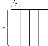
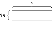
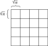
Figure 1: Vertical slices (a), horizontal slices (b), and blocks (c)
Algorithm rotatesort is based on three operations: balance, unblock and shear.
balance
Operation balance is applied to a vertical slice.
- Sort the columns
- Rotate the rows
- Sort the columns
Each row i is rotated by i mod  n positions.
unblock
Operation unblock is applied to the whole array. It distributes the n elements of each block over the whole width of the array.
- Rotate the rows
- Sort the columns
Each row i of the arrayis rotated by i· n mod n positions.
shear
Operation shear is applied to the whole array.
- Sort the rows in alternating direction
- Sort the columns
Sorting in alternating direction means that each row i is sorted in ascending order if i is even, and in descending order if i is odd.
Algorithm rotatesort
Input:
unsorted n×n-array of data
Output:
sorted n×n-array
Method:
- balance each vertical slice;
- unblock;
- balance each horizontal slice;
- unblock;
- shear three times;
- sort the rows;
In Step 3 balance is applied to a horizontal slice as if it were a vertical slice lying on its side.
Correctness
The correctness of algorithm rotatesort is shown using the 0-1-principle. In the following figures zeroes are drawn in white and ones in gray.
Definition: An r×s-subarray is called clean, if it consists of zeroes or ones only, respectively. Otherwise it is called dirty.
In particular, this definition refers to rows and blocks. A dirty row contains zeroes as well as ones, a clean row contains either zeroes or ones.
Step 1
Operation balance, applied to a vertical slice, reduces the number of dirty rows in the slice to at most  n. This is the case because after sorting the columns in step (a), each column of the slice is distributed to all columns of the slice by the rotation in step (b). After sorting the columns again in step (c), the 1's of each column contribute to a certain number of clean 1-rows and, possibly, a dirty row (Figure 2).
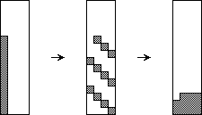
Figure 2: Distributing the 1's of a column by operation balance
Since each of the  n columns of the slice can generate a dirty row there remain at most
  n dirty rows in the slice. The dirty rows of a slice span across at most two blocks.
Altogether, there remain at most 2 n dirty blocks after Step 1. This situation is shown in Figure 3.
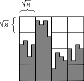
Figure 3: Situation after Step 1
Step 2
Operation unblock distributes each block to all columns by the rotation in step (a) (Figure 4).
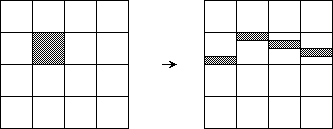
Figure 4: Rotation of operation unblock
By sorting the columns in step (b) each clean block generates a clean row and each dirty block generates a dirty row. Therefore, at most 2 n dirty rows that stem from the at most 2
 n dirty blocks remain after Step 2.
Step 3
The at most 2 n dirty rows contribute to at most three horizontal slices. After Step 3 (balance applied to the horizontal slices) there remain at most 6 dirty blocks (Figure 5).
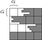
Figure 5: Situation after Step 3
Step 4
Step 4 (unblock) distributes the at most 6 dirty blocks to at most 6 dirty rows.
Step 5
Operation shear reduces every two dirty rows to at most one dirty row. After sorting the rows in alternating direction, the odd rows start with zeroes and end with ones, the even rows start with ones and end with zeroes. By sorting the columns a clean row of zeroes (Figure 6a) or a clean row of ones (Figure 6b) is produced from every two dirty rows.


Figure 6: Operation shear
This technique is also applied in algorithm shearsort [SchS 89], as well as in algorithm 4-way mergesort [Schi 87].
By the operation shear the number of dirty rows is halved. By the threefold application of shear in Step 5 the 6 dirty rows are reduced to one dirty row.
Step 6
Eventually, in Step 6 the last remaining dirty row is sorted.
We have shown that the algorithm sorts all 0-1-data sequences. Due to the 0-1-principle, it therefore sorts every arbitrary data sequence.
Analysis
The analysis of rotatesort yields the following number of phases, where sorting or rotating a row or column, respectively, is preliminarily counted as a phase.
| Step 1: | balance | 3 | phases | |||
| Step 2: | unblock | 2 | phases | |||
| Step 3: | balance | 3 | phases | |||
| Step 4: | unblock | 2 | phases | |||
| Step 5: | 3 × shear | 6 | phases | |||
| Step 6: | sorting the rows | 1 | phase | |||
| altogether: | 17 | phases |
Since a phase is a maximal sequence of row or column operations, this value decreases to 16, because step 3c and step 4a both apply to rows.
If sorting of a row or column is performed with odd-even transposition sort, and if rotation is realized with local exchanges as well, each phase requires at most n elementary steps. The algorithm therefore is in O(n), but the constant of 17 is rather poor. For instance, algorithm 4-way mergesort has a constant of 7. The lower bound is 3 (neglecting low order terms), and it is attained by the algorithms of Thompson/Kung [TK 77] and Schnorr/Shamir [SchSh 86].
By a more careful analysis the constant is reduced to 10 (plus low order terms). In Step 1 and Step 3 the rotation phases need not be counted, since they require only  n elementary steps. The rotation phase of unblock can be realized in n/2 elementary steps by implementing a right rotation of k > n/2 positions by a left rotation of n-k < n/2 positions. In Step 4 unblock produces at most 3
 n dirty rows; thus a corresponding number of odd-even transposition sort steps suffices for sorting the columns. Moreover, sorting the columns in shear requires only a constant number of odd-even transposition sort steps, since there is only a constant number of dirty rows. These phases need not be counted.
Theorem: Rotatesort requires at most 10n + O( n) elementary steps.
Simulation
The following applet shows execution of rotatesort with a 64×64-array of zeroes and ones. For illustration row and column operations are shown sequentially that would be performed in parallel on a two-dimensional processor array.
(Java applet for simulation of rotatesort)
Conclusions
Algorithm rotatesort for sorting an n×n-array has the same asymptotic time complexity as the algorithm of Thompson/Kung [TK 77], namely O(n). Regarding the constant, it is slower by a factor of about 3. The quality of the algorithm lies in its simplicity while being asymptoticly optimal at the same time.
References
[MG 88] J.M. Marberg, E. Gafni: Sorting in Constant Number of Row and Column Phases on a Mesh. Algorithmica 3, 561-572 (1988)
[Schi 87] M. Schimmler: Fast Sorting on the Instruction Systolic Array. Bericht Nr. 8709, Institut für Informatik, Christian-Albrechts-Universität Kiel (1987)
[SchS 89] I.D. Scherson, S. Sen: Parallel sorting in two-dimensional VLSI models of computation. IEEE Transactions on Computers C-38, 2, 238-249 (1989)
[SchSh 86] C.P. Schnorr, A. Shamir: An Optimal Sorting Algorithm for Mesh-Connected Computers. Proc. of the 18th ACM Symposium on Theory of Computing, 255-261 (1986)
[TK 77] C.D. Thompson, H.T. Kung: Sorting on a Mesh-Connected Parallel Computer. Communications of the ACM, 20, 4, 263-271 (1977)
Next: [Sorting algorithm of Schnorr/Shamir] or [up]
H.W. Lang mail@hwlang.de Impressum Datenschutz
Created: 16.05.2001 Updated: 07.02.2023